Database, Models, and Metadata
Models
The core functionality of pyrrhenius is used via pyrrhenius.model.ModelInterface objects. While you can certainty instantiate your own, pyrrhenius.model.ModelInterface’s are more easily obtained through interaction with a
pyrrhenius.database.Database object as described in the quickstart and database sections.
pyrrhenius.model.ModelInterface objects have a number of useful methods and attributes. One of these is the pyrrhenius.model.ModelInterface.metadata attribute, which is integrated into the model to allow automatic error-checking when using the model to calculate electric conductivity.
pyrrhenius.model.ModelInterface objects can also be combined with the + operator, resulting in a linear combination of the two models. This is useful when integtrating say, a proton diffusion model with an electronic conduction model:
nv17HD  = ecdatabase.get_model('nv_17_ol[010]') # Novella et al. 2017's hydrogen diffusion equation
print(nv17HD)

seo3dry =  ecdatabase.get_model('SEO3_ol') # Constable et al. 2006's dry olivine equation
print(seo3dry)

combined = nv17HD+seo3dry
print(combined)
nv_17_ol[010]:{1.8e+42(nan) Cw * 10^-5.0(0.9) * exp(1.782654381(0.196921123)/kT)/kT}
SEO3_ol:{e*(5.06e+24(nan) exp( -0.357(nan)/kT) 3.33e+24(nan) exp( -0.02(nan)/kT) fO2^0.166667(nan))*1.22e-05(nan) exp( -1.05(nan)/kT) + e*(4.58e+26(nan) exp( -0.752(nan)/kT) 6.209999999999999e+30(nan) exp( -1.83(nan)/kT) fO2^0.166666667(nan))*5.44e-06(nan) exp( -1.09(nan)/kT)}
nan bell (2003)
nan ppm
nan nan
nan bell (2003)
nan ppm
nan nan
nan bell (2003)
nan ppm
nan nan
{nv_17_ol[010]+SEO3_ol}
As may be apparent, calling the __repr__ method by casting the models to strings reveals both the underlying model_id and a string representation of the arrhenian form. More details are provided on what this string forms represents below and in the API section.
Calculating Conductivity
The function you will use the most on your model objects is get_conductivity(), which tells the underlying model to calculate electric conductivity. Models implicitly vectorize computations to match the largest dimension size of the provided keyword-arguments.
model = ecdatabase.get_model('SEO3_ol')
model.get_conductivity(T=1000, P=1.0, logfo2=10**-11)
2.7380861532827377e-05
T = np.ones(4)*700 # in degrees K
print(T.shape)
model.get_conductivity(T=T, P=1.0, logfo2=10**-11)
(4,)
array([1.29536636e-07, 1.29536636e-07, 1.29536636e-07, 1.29536636e-07])
T = np.ones((4,4))*700 # in degrees K
print(T.shape)
model.get_conductivity(T=T, P=1.0, logfo2=10**-11)
(4, 4)
array([[1.29536636e-07, 1.29536636e-07, 1.29536636e-07, 1.29536636e-07],
       [1.29536636e-07, 1.29536636e-07, 1.29536636e-07, 1.29536636e-07],
       [1.29536636e-07, 1.29536636e-07, 1.29536636e-07, 1.29536636e-07],
       [1.29536636e-07, 1.29536636e-07, 1.29536636e-07, 1.29536636e-07]])
keywords provided as np.ndarray’s can either be all the same shape, a mixture of one shape and floats, or a mixture of one shape, floats, and arrays of shape (1,)
In the prior example, the keywords T for temperature, P for pressure, and logfo2 were provided to the pyrrhenius.model.Model instance corresponding to the SEO3 model of olivine. This model notably requires pressure and oxygen fugacity to calculate electrical conductivity.
If we tried to run the SEO3 model without these keywords pyrrhenius will inform you that they need to be provided
try:
    model.get_conductivity(T=T)
except AssertionError as e:
    print(e)
logfo2 not provided. Pass logfo2 as a keyword-argument
code in both the underlying pyrrhenius.mechanism.Mechanism and pyrrhenius.model.Model classes is designed to raise an error if required keywords are not provided.
if you are unsure what keywords need to be provided to a model object, the print_required_parameters() method will tell you
model.print_required_parameters()******************** Required Keywords ******************** Intrinsic Arguments -------------------- Volatile Arguments -------------------- Electronic Conduction Arguments -------------------- *logfo2 Diffusion Conduction Arguments -------------------- Polymerizing Agent Arguments --------------------
Note that currently temperature is a required keyword-argument for all models, even static valued ones.
The following table lists the keyword-arguments currently accepted by pyrrhenius along with the required unit conventions.
Parameter |
Keyword-argument |
Units |
|---|---|---|
Temperature |
T |
Kelvin |
Pressure |
P |
GPa |
Oxygen fugacity |
logfo2 |
\(\log_{10}(bars)\) |
Water concentration |
Cw |
ppm wt% |
Carbon dioxide |
co2 |
wt% |
Sodium Chloride |
nacl |
wt% |
Silicon Dioxide |
sio2 |
wt% |
Iron Fraction |
X_fe |
normalized fraction (typically Fe/(Mg+Fe)) |
Basic Anisotropic Models
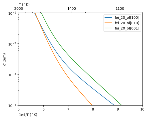
Some laboratory experiments have documented conductivities which depend on crystallographic orientation. This is especially true of olivine, which has seen considerable research interest over the last 40 years due to its abundance in the Earth’s upper mantle.
Lets see what Pyrrhenius identifiers exist for olivine:
import pyrrhenius.database as phsd

ecdatabase = phsd.Database()

ecdatabase.get_model_list_for_phase('olivine')
['SEO2_ol', 'xu_2000_ol[001]', 'xu_2000_ol[010]', 'xu_2000_ol[100]', 'xu_2000_poly_ol', 'dF_05_ol[100]', 'dF_05_ol[010]', 'dF_05_ol[001]', 'SEO3_ol', 'wang_06_ol', 'dk_2009_ol', 'ty_09_dry_ol', 'ty_09_ol', 'ty_12_ol', 'yang_12b_ol[100]', 'yang_12b_ol[010]', 'yang_12b_ol[001]', 'gar_14_bell_ol[100]', 'gar_14_bell_ol[010]', 'gar_14_bell_ol[001]', 'gar_14_withers_ol[100]', 'gar_14_withers_ol[010]', 'gar_14_withers_ol[001]', 'y_16_ol[100]', 'y_16_ol[010]', 'y_16_ol[001]', 'nv_17_ol[100]', 'nv_17_ol[010]', 'nv_17_ol[001]', 'sun_19ol[100]', 'sun_19ol[001]', 'fei_20_ol[100]', 'fei_20_ol[010]', 'fei_20_ol[001]', 'fei_20_ol_ionic[100]', 'fei_20_ol_ionic[010]', 'fei_20_ol_ionic[001]']
Scrolling through the list, you should see some models which have the string [xxx] appended to the end. Each represents a parameterization for a separate crystallographic direction. For example, the fei_20_ol model actually has three possible models associated with it, fei_20_ol[100], fei_20_ol[010], and fei_20_ol[001].
import matplotlib.pyplot as plt
import numpy as np
import pyrrhenius.database as phsd
import pyrrhenius.utils as pyhutils

ecdatabase = phsd.Database()

models = ['fei_20_ol[100]','fei_20_ol[010]', 'fei_20_ol[001]']


T = np.linspace(400,1800,num=120) # temperature in kelvin

fig, ax = plt.subplots()
linear_major_ticks = np.asarray([2000,1400,1100,900,800,700,600,500,400])
pyhutils.format_ax_arrhenian_space(ax,linear_major_ticks=linear_major_ticks,xlim=[5,10])
Cw = 100 # 100 ppm water
P = 3 # 3 GPa
for model_id in models:
    ecmodel = ecdatabase.get_model(model_id)
    c = ecmodel.get_conductivity(T=T,Cw=Cw,P=P)
    ax.plot(1e4/T,c,label=model_id)
ax.legend()
ax.set_ylim([1e-4,1e-1])
fig.show()
Be careful though! Many of the isotropic models contained in the default database are specific to high-temperature mechanisms, relying on other published works to provide the low-temperature mechanisms. There are easy ways to deal with model mixing and matching, which is elaborated upon in the Special Model Section.
Derived Isotropic Models and Advanced Anisotropy
In some cases, publications may not have provided an isotropic parameterization, or perhaps you, the user, wants to estimate the isotropic conductivity based on your own models. Pyrrhenius provides a functionality for automatically creating isotropic variants of existing anisotropic models. Simply call database.create_isotropic_models() and
the pyrrhenius database object will internally create its own isotropic representation of every anisotropic model within the database. Printing out the list of available isotropic models shows that new models have been added which have a prefix of isotropic_model:...
ecdatabase = phsd.Database()
ecdatabase.create_isotropic_models()
ecdatabase.get_model_list_for_phase('olivine')[-12:]
nan nan
nan nan
nan nan
nan nan
nan nan
nan nan
nan nan
nan nan
nan nan
nan nan
nan nan
nan nan
nan nan
nan nan
nan nan
nan nan
nan nan
nan nan
withers (2012) withers (2012)
ppm ppm
nan nan
withers (2012) withers (2012)
ppm ppm
nan nan
withers (2012) withers (2012)
ppm ppm
nan nan
withers (2012) withers (2012)
ppm ppm
nan nan
withers (2012) withers (2012)
ppm ppm
nan nan
withers (2012) withers (2012)
ppm ppm
nan nan
withers (2012) withers (2012)
ppm ppm
nan nan
withers (2012) withers (2012)
ppm ppm
nan nan
withers (2012) withers (2012)
ppm ppm
nan nan
withers (2012) withers (2012)
ppm ppm
nan nan
withers (2012) withers (2012)
ppm ppm
nan nan
withers (2012) withers (2012)
ppm ppm
nan nan
withers (2012) withers (2012)
ppm ppm
nan nan
withers (2012) withers (2012)
ppm ppm
nan nan
withers (2012) withers (2012)
ppm ppm
nan nan
withers (2012) withers (2012)
ppm ppm
nan nan
withers (2012) withers (2012)
ppm ppm
nan nan
withers (2012) withers (2012)
ppm ppm
nan nan
withers (2012) withers (2012)
ppm ppm
nan nan
withers (2012) withers (2012)
ppm ppm
nan nan
withers (2012) withers (2012)
ppm ppm
nan nan
withers (2012) withers (2012)
ppm ppm
nan nan
withers (2012) withers (2012)
ppm ppm
nan nan
withers (2012) withers (2012)
ppm ppm
nan nan
nan nan
nan nan
nan nan
nan nan
nan nan
nan nan
nan nan
nan nan
nan nan
nan nan
nan nan
nan nan
nan nan
nan nan
nan nan
nan nan
nan nan
nan nan
nan nan
nan nan
nan nan
nan nan
nan nan
nan nan
nan nan
nan nan
nan nan
bell (2003) bell (2003)
ppm ppm
nan nan
bell (2003) bell (2003)
ppm ppm
nan nan
bell (2003) bell (2003)
ppm ppm
nan nan
bell (2003) bell (2003)
ppm ppm
nan nan
bell (2003) bell (2003)
ppm ppm
nan nan
bell (2003) bell (2003)
ppm ppm
nan nan
paterson (1982) paterson (1982)
wtpct wtpct
nan nan
paterson (1982) paterson (1982)
wtpct wtpct
nan nan
paterson (1982) paterson (1982)
wtpct wtpct
nan nan
paterson (1982) paterson (1982)
wtpct wtpct
nan nan
paterson (1982) paterson (1982)
wtpct wtpct
nan nan
paterson (1982) paterson (1982)
wtpct wtpct
nan nan
paterson (1982) paterson (1982)
ppm ppm
nan nan
paterson (1982) paterson (1982)
ppm ppm
nan nan
paterson (1982) paterson (1982)
ppm ppm
nan nan
nan nan
nan nan
nan nan
nan nan
nan nan
nan nan
nan nan
nan nan
nan nan
nan nan
nan nan
nan nan
nan nan
nan nan
nan nan
nan nan
nan nan
nan nan
Libowitzky and rossman (1996) Libowitzky and rossman (1996)
wtpct wtpct
nan nan
Libowitzky and rossman (1996) Libowitzky and rossman (1996)
wtpct wtpct
nan nan
Libowitzky and rossman (1996) Libowitzky and rossman (1996)
wtpct wtpct
nan nan
Libowitzky and rossman (1996) Libowitzky and rossman (1996)
wtpct wtpct
nan nan
Libowitzky and rossman (1996) Libowitzky and rossman (1996)
wtpct wtpct
nan nan
Libowitzky and rossman (1996) Libowitzky and rossman (1996)
wtpct wtpct
nan nan
nan nan
nan nan
nan nan
nan nan
nan nan
nan nan
nan nan
nan nan
nan nan
nan nan
nan nan
nan nan
nan nan
nan nan
nan nan
nan nan
nan nan
nan nan
bell (1995) bell (1995)
ppm ppm
nan nan
bell (1995) bell (1995)
ppm ppm
nan nan
bell (1995) bell (1995)
ppm ppm
nan nan
bell (1995) bell (1995)
ppm ppm
nan nan
bell (1995) bell (1995)
ppm ppm
nan nan
bell (1995) bell (1995)
ppm ppm
nan nan
bell (2003) bell (2003)
ppm ppm
nan nan
bell (2003) bell (2003)
ppm ppm
nan nan
bell (2003) bell (2003)
ppm ppm
nan nan
bell (2003) bell (2003)
ppm ppm
nan nan
bell (2003) bell (2003)
ppm ppm
nan nan
bell (2003) bell (2003)
ppm ppm
nan nan
Johnson and Rossman (2003) Johnson and Rossman (2003)
ppm ppm
nan nan
Johnson and Rossman (2003) Johnson and Rossman (2003)
ppm ppm
nan nan
Johnson and Rossman (2003) Johnson and Rossman (2003)
ppm ppm
nan nan
Johnson and Rossman (2003) Johnson and Rossman (2003)
ppm ppm
nan nan
Johnson and Rossman (2003) Johnson and Rossman (2003)
ppm ppm
nan nan
Johnson and Rossman (2003) Johnson and Rossman (2003)
ppm ppm
nan nan
['fei_20_ol_ionic[010]',
 'fei_20_ol_ionic[001]',
 'isotropic_model:dF_05_ol[100]+dF_05_ol[010]+dF_05_ol[001]',
 'isotropic_model:fei_20_ol[100]+fei_20_ol[010]+fei_20_ol[001]',
 'isotropic_model:fei_20_ol_ionic[100]+fei_20_ol_ionic[010]+fei_20_ol_ionic[001]',
 'isotropic_model:gar_14_bell_ol[100]+gar_14_bell_ol[010]+gar_14_bell_ol[001]',
 'isotropic_model:gar_14_withers_ol[100]+gar_14_withers_ol[010]+gar_14_withers_ol[001]',
 'isotropic_model:nv_17_ol[100]+nv_17_ol[010]+nv_17_ol[001]',
 'isotropic_model:sun_19ol[100]+sun_19ol[001]',
 'isotropic_model:xu_2000_ol[001]+xu_2000_ol[010]+xu_2000_ol[100]',
 'isotropic_model:y_16_ol[100]+y_16_ol[010]+y_16_ol[001]',
 'isotropic_model:yang_12b_ol[100]+yang_12b_ol[010]+yang_12b_ol[001]']
Use of these is similar to previous models
fig, ax = plt.subplots()
linear_major_ticks = np.asarray([2000,1400,1100,900,800,700,600,500,400])
pyhutils.format_ax_arrhenian_space(ax,linear_major_ticks=linear_major_ticks,xlim=[5,10])
Cw = 100 # 100 ppm water
P = 3 # 3 GPa
for model_id in models:
    ecmodel = ecdatabase.get_model(model_id)
    c = ecmodel.get_conductivity(T=T,Cw=Cw,P=P)
    ax.plot(1e4/T,c,label=model_id)

isotropic_model_id = 'isotropic_model:fei_20_ol[100]+fei_20_ol[010]+fei_20_ol[001]'
ecmodel = ecdatabase.get_model(isotropic_model_id)
c = ecmodel.get_conductivity(T=T,Cw=Cw,P=P)
ax.plot(1e4/T,c,label=model_id,linestyle='--',color='blue')
ax.legend()
ax.set_ylim([1e-4,1e-1])
fig.show()
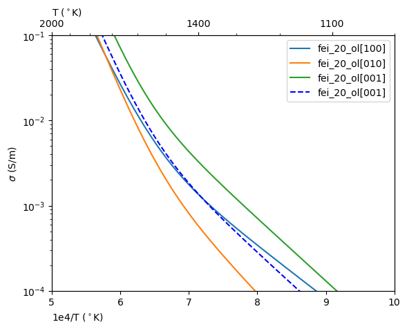
These derived models utilize a geometric mean to calculate the isotropic conductivity by assuming each crystal direction makes up \(1/N\) of the total substance, where N represents the number of crystallographic orientations available per id.
Derived isotropic models allow for dynamic querying of isotropic parameters through a number of options specified by the averaging keyword argument in the method get_conductivity. The available options for averaging include:
Geometric Mean (default): Example usage:
Cw = 100 # 100 ppm water
P = 3 # 3 GPa
T = np.linspace(1000,1500,num=10)
physiokwargs = {'Cw':Cw,'P':P,'T':T}
conductivity = ecmodel.get_conductivity(**physiokwargs)
conductivity
array([9.54131586e-06, 2.32192181e-05, 5.17208096e-05, ...,
       1.21434816e-03, 2.18061769e-03, 4.07701613e-03])
Max Anisotropic Conductivity: By setting
averagingto'max_aniso', the method returns the conductivity in the most conductive direction
conductivity = ecmodel.get_conductivity(averaging='max_aniso',**physiokwargs)
conductivity
array([2.40550310e-05, 5.85447366e-05, 1.30385620e-04, ...,
       2.92689511e-03, 5.07132817e-03, 9.06025978e-03])
Min Anisotropic Conductivity: When
averagingis set to'min_aniso', the method returns the conductivity in the least conductive direction
conductivity = ecmodel.get_conductivity(averaging='min_aniso',**physiokwargs)
conductivity
array([1.85038547e-06, 5.17375901e-06, 1.30593207e-05, ...,
       5.02547241e-04, 9.90020304e-04, 2.03826257e-03])
In addition to these averaging methods, the method supports querying for a specific crystal direction by passing the crystal_direction argument. If a crystal direction is specified and found within the available crystallographic directions, the method will return the conductivity for that specific direction.
conductivity = ecmodel.get_conductivity(crystal_direction='[100]',**physiokwargs)
conductivity
array([1.95144667e-05, 4.13284124e-05, 8.12541700e-05, ...,
       1.21743450e-03, 2.06525070e-03, 3.66966574e-03])
Alternatively, you can provide a float value between 0 and 1. In this case, the method will return an anisotropic factor corresponding to the given ratio between the minimum and maximum conductivities. This ratio represents the interpolation between the most and least conductive directions, calculated by the following equation
Where:
\(\sigma_{\text{anisotropic}}\) is the resulting conductivity based on the factor.
\(\sigma_{\text{min}}\) is the conductivity in the least conductive direction.
\(\sigma_{\text{max}}\) is the conductivity in the most conductive direction.
f is the float value between 0 and 1 representing the desired anisotropic ratio.
conductivity = ecmodel.get_conductivity(crystal_direction=0.5,**physiokwargs)
conductivity
array([1.29527083e-05, 3.18592478e-05, 7.17224706e-05, ...,
       1.71472118e-03, 3.03067424e-03, 5.54926118e-03])
The anisotropic factor can also be provided as a np.ndarray, as long as it has the same dimensions as other physiochemical variables. This allows for querying anisotropic conductivity across multiple values simultaneously.
import numpy as np

# Provide an array of anisotropic factors for batch querying
factors = np.random.uniform(0,1,size=len(T))
print(f'Anisotropic Factors: {factors}')
conductivity = ecmodel.get_conductivity(crystal_direction=factors,**physiokwargs)
conductivity
Anisotropic Factors: [0.41393503 0.11618761 0.50551 ... 0.20663594 0.74778231 0.3740369 ]
array([1.10416660e-05, 1.13748054e-05, 7.23689379e-05, ...,
       1.00350464e-03, 4.04195014e-03, 4.66474865e-03])
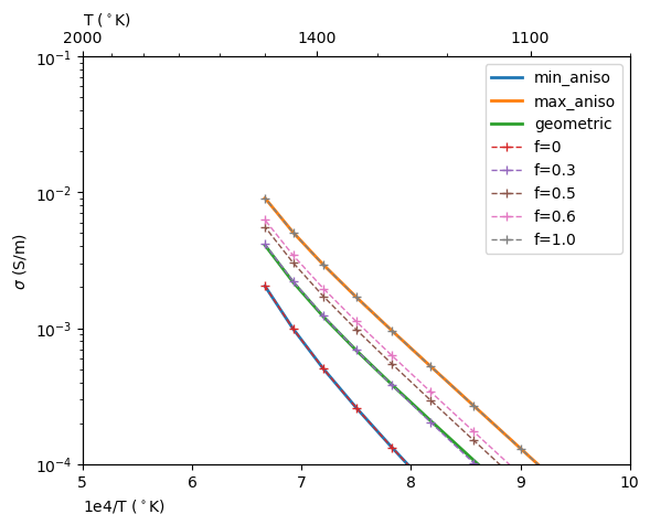
By combining these lessons we can see these shortcuts allow us to interrogate anisotropic behavior of a derived model with less code and less knowledge of the pyrrhenius id’s.
fig, ax = plt.subplots()
linear_major_ticks = np.asarray([2000,1400,1100,900,800,700,600,500,400])
pyhutils.format_ax_arrhenian_space(ax,linear_major_ticks=linear_major_ticks,xlim=[5,10])

# Physiochemical states
Cw = 100 #(100 ppm water)
P = 3 # 3 GPa
T = np.linspace(1000,1500,num=10)
physiokwargs = {'Cw':Cw,'P':P,'T':T}


isotropic_model_id = 'isotropic_model:fei_20_ol[100]+fei_20_ol[010]+fei_20_ol[001]'
ecmodel = ecdatabase.get_model(isotropic_model_id)

for averaging in ['min_aniso','max_aniso','geometric']:
    c = ecmodel.get_conductivity(averaging=averaging,**physiokwargs)
    print(c)
    print(1e4/T)
    ax.plot(1e4/T,c,label=averaging,linewidth=2)

for factor in [0,0.3,0.5,0.6,1.0]:
    c = ecmodel.get_conductivity(crystal_direction=factor,**physiokwargs)
    ax.plot(1e4/T,c,label=f'f={factor}',linestyle='--',linewidth=1,marker='+')
ax.legend()
ax.set_ylim([1e-4,1e-1])
fig.show()
[1.85038547e-06 5.17375901e-06 1.30593207e-05 ... 5.02547241e-04
 9.90020304e-04 2.03826257e-03]
[10.          9.47368421  9.         ...  7.2         6.92307692
  6.66666667]
[2.40550310e-05 5.85447366e-05 1.30385620e-04 ... 2.92689511e-03
 5.07132817e-03 9.06025978e-03]
[10.          9.47368421  9.         ...  7.2         6.92307692
  6.66666667]
[9.54131586e-06 2.32192181e-05 5.17208096e-05 ... 1.21434816e-03
 2.18061769e-03 4.07701613e-03]
[10.          9.47368421  9.         ...  7.2         6.92307692
  6.66666667]
Note
As seen on the graph, an anisotropic factor of f=0.5 is not equal to the geometric mean.
Special Models
The Pyrrhenius models used so far are relatively basic, but there are easy ways to combine them to achieve specific functionalities. At the time of this writing, three types of models are available,
Composite Models: Used to combine multiple arrhenian mechanisms or multiple publications together
Water Correction Models: Used to modify the water value either to the whole model or to only certain mechanisms of a composite model.
Cached Models: Used when calculating the electric conductivity of a substance is time-consuming and likely to result in the same value over repeated calls.
Composite Models
Composite models are used to combine multiple physical mechanisms or correction factors into a single model. These are useful in cases where a single mechanism or single experimental result isn’t sufficient to replicate electric conductivity.
Consider the fei_20_ol_ionic[xxx] models and the nv_17_ol[xxx] models. Both of these experiments report mechanism parameterizations which are meant to be added to lower temperature or dry olivine experiments. Lets assume that the SEO3 model of olivine from Constable, (2006) will be the dry/low temperature model of choice.
from pyrrhenius.database import Database

ecdatabase = Database()

dry_model = ecdatabase.get_model('SEO3_ol')
novella_models =['nv_17_ol[100]','nv_17_ol[010]','nv_17_ol[001]']
fei_models = ['fei_20_ol_ionic[100]','fei_20_ol_ionic[010]', 'fei_20_ol_ionic[001]']
To create the composite model, I’ll loop over each model, add via the + operator the dry model to a novella or fei model, then register the new object by calling .register_new_model() the database
from pyrrhenius.utils import calc_QFM
T = np.linspace(1000,2300,num=10) # in K
P = np.linspace(3,10,num=10) # in GPa
qfm = calc_QFM(T,P)
Cw = 300 # (in ppm)
physiochem = {'T':T,'P':P,'Cw':Cw,'logfo2':qfm}
models_to_composite = novella_models+fei_models

for id in models_to_composite:
    print('*'*20)
    print(id)
    ecmodel = ecdatabase.get_model(id)
    print(ecmodel.get_conductivity(**physiochem))
    new_ecmodel = ecmodel + dry_model
    print(new_ecmodel.get_conductivity(**physiochem))
    print(f'old ec model representation:{ecmodel}')
    print(f'new ec model representation:{new_ecmodel}')
    ecdatabase.register_new_model(new_ecmodel)
********************
nv_17_ol[100]
[3.50705631e-05 9.90950092e-04 1.30542793e-02 ... 1.80010978e+01
 4.20468535e+01 8.79148355e+01]
nan bell (2003)
nan ppm
nan nan
nan bell (2003)
nan ppm
nan nan
nan bell (2003)
nan ppm
nan nan
[3.62561072e-05 1.00357414e-03 1.31427507e-02 ... 1.83972555e+01
 4.37197301e+01 9.39204533e+01]
old ec model representation:nv_17_ol[100]:{1.8e+42(nan) Cw * 10^-0.7(0.9) * exp(2.373417751(0.186556854)/kT)/kT}
new ec model representation:{nv_17_ol[100]+SEO3_ol}
********************
nv_17_ol[010]
[1.66824213e-06 1.98422234e-05 1.33579471e-04 ... 2.72729762e-02
 5.06947206e-02 8.68055584e-02]
nan bell (2003)
nan ppm
nan nan
nan bell (2003)
nan ppm
nan nan
nan bell (2003)
nan ppm
nan nan
[2.85378621e-06 3.24662702e-05 2.22050961e-04 ... 4.23430675e-01
 1.72357132e+00 6.09242337e+00]
old ec model representation:nv_17_ol[010]:{1.8e+42(nan) Cw * 10^-5.0(0.9) * exp(1.782654381(0.196921123)/kT)/kT}
new ec model representation:{nv_17_ol[010]+SEO3_ol}
********************
nv_17_ol[001]
[7.70053971e-06 1.16770705e-04 9.49122714e-04 ... 3.31262475e-01
 6.56521973e-01 1.18900374e+00]
nan bell (2003)
nan ppm
nan nan
nan bell (2003)
nan ppm
nan nan
nan bell (2003)
nan ppm
nan nan
[8.88608380e-06 1.29394752e-04 1.03759420e-03 ... 7.27420174e-01
 2.32939857e+00 7.19462156e+00]
old ec model representation:nv_17_ol[001]:{1.8e+42(nan) Cw * 10^-3.5(0.4) * exp(1.948482695(0.082914157)/kT)/kT}
new ec model representation:{nv_17_ol[001]+SEO3_ol}
********************
fei_20_ol_ionic[100]
[7.23469940e-09 9.04702653e-07 3.77916203e-05 ... 1.38987350e+00
 4.80779309e+00 1.41706718e+01]
nan withers (2012)
nan ppm
nan nan
nan withers (2012)
nan ppm
nan nan
nan withers (2012)
nan ppm
nan nan
[1.19277878e-06 1.35287494e-05 1.26263111e-04 ... 1.78603120e+00
 6.48066969e+00 2.01762897e+01]
old ec model representation:fei_20_ol_ionic[100]:{Cw^1.3(0.2) 10^9.9(5.00E-01) exp(-(3.492758874(0.155464045) + P4.2(0.4))/kT)/T}
new ec model representation:{fei_20_ol_ionic[100]+SEO3_ol}
********************
fei_20_ol_ionic[010]
[4.30852962e-10 1.36803548e-07 1.17751141e-05 ... 3.38772410e+00
 1.49869656e+01 5.47740243e+01]
nan withers (2012)
nan ppm
nan nan
nan withers (2012)
nan ppm
nan nan
nan withers (2012)
nan ppm
nan nan
[1.18597494e-06 1.27608503e-05 1.00246605e-04 ... 3.78388180e+00
 1.66598422e+01 6.07796421e+01]
old ec model representation:fei_20_ol_ionic[010]:{Cw^1.3(0.2) 10^11.6(4.00E-01) exp(-(4.104250784(0.259106741) + P3.2(0.2))/kT)/T}
new ec model representation:{fei_20_ol_ionic[010]+SEO3_ol}
********************
fei_20_ol_ionic[001]
[1.76960339e-09 4.60233007e-07 3.39315979e-05 ... 6.28384594e+00
 2.63725119e+01 9.20463369e+01]
nan withers (2012)
nan ppm
nan nan
nan withers (2012)
nan ppm
nan nan
nan withers (2012)
nan ppm
nan nan
[1.18731369e-06 1.30842797e-05 1.22403088e-04 ... 6.68000363e+00
 2.80453885e+01 9.80519547e+01]
old ec model representation:fei_20_ol_ionic[001]:{Cw^1.3(0.2) 10^11.78(4.00E-01) exp(-(3.990243818(0.155464045) + P4.1(0.4))/kT)/T}
new ec model representation:{fei_20_ol_ionic[001]+SEO3_ol}
While right now the representations are a bit wordy, it should be evident the new ec model was created by examining the new SEO3.. string added to the representation.
Similar to before, creation of a new derived isotropic model can be done by calling .create_isotropic_models() on the existing database object
ecdatabase.create_isotropic_models()
model_list = ecdatabase.get_model_list_for_phase('olivine')
model_list[-20:]
nan nan
nan nan
nan nan
nan nan
nan nan
nan nan
nan nan
nan nan
nan nan
nan nan
nan nan
nan nan
nan nan
nan nan
nan nan
nan nan
nan nan
nan nan
withers (2012) withers (2012)
ppm ppm
nan nan
withers (2012) withers (2012)
ppm ppm
nan nan
withers (2012) withers (2012)
ppm ppm
nan nan
withers (2012) withers (2012)
ppm ppm
nan nan
withers (2012) withers (2012)
ppm ppm
nan nan
withers (2012) withers (2012)
ppm ppm
nan nan
withers (2012) withers (2012)
ppm ppm
nan nan
withers (2012) withers (2012)
ppm ppm
nan nan
withers (2012) withers (2012)
ppm ppm
nan nan
withers (2012) withers (2012)
ppm ppm
nan nan
withers (2012) withers (2012)
ppm ppm
nan nan
withers (2012) withers (2012)
ppm ppm
nan nan
nan nan
nan nan
nan nan
nan nan
nan nan
nan nan
nan nan
nan nan
nan nan
nan nan
nan nan
nan nan
nan nan
nan nan
nan nan
nan nan
nan nan
nan nan
withers (2012) withers (2012)
ppm ppm
nan nan
withers (2012) withers (2012)
ppm ppm
nan nan
withers (2012) withers (2012)
ppm ppm
nan nan
withers (2012) withers (2012)
ppm ppm
nan nan
withers (2012) withers (2012)
ppm ppm
nan nan
withers (2012) withers (2012)
ppm ppm
nan nan
withers (2012) withers (2012)
ppm ppm
nan nan
withers (2012) withers (2012)
ppm ppm
nan nan
withers (2012) withers (2012)
ppm ppm
nan nan
withers (2012) withers (2012)
ppm ppm
nan nan
withers (2012) withers (2012)
ppm ppm
nan nan
withers (2012) withers (2012)
ppm ppm
nan nan
nan nan
nan nan
nan nan
nan nan
nan nan
nan nan
nan nan
nan nan
nan nan
nan nan
nan nan
nan nan
nan nan
nan nan
nan nan
nan nan
nan nan
nan nan
nan nan
nan nan
nan nan
nan nan
nan nan
nan nan
nan nan
nan nan
nan nan
bell (2003) bell (2003)
ppm ppm
nan nan
bell (2003) bell (2003)
ppm ppm
nan nan
bell (2003) bell (2003)
ppm ppm
nan nan
bell (2003) bell (2003)
ppm ppm
nan nan
bell (2003) bell (2003)
ppm ppm
nan nan
bell (2003) bell (2003)
ppm ppm
nan nan
nan nan
nan nan
nan nan
nan nan
nan nan
nan nan
nan nan
nan nan
nan nan
nan nan
nan nan
nan nan
nan nan
nan nan
nan nan
nan nan
nan nan
nan nan
paterson (1982) paterson (1982)
wtpct wtpct
nan nan
paterson (1982) paterson (1982)
wtpct wtpct
nan nan
paterson (1982) paterson (1982)
wtpct wtpct
nan nan
paterson (1982) paterson (1982)
wtpct wtpct
nan nan
paterson (1982) paterson (1982)
wtpct wtpct
nan nan
paterson (1982) paterson (1982)
wtpct wtpct
nan nan
paterson (1982) paterson (1982)
ppm ppm
nan nan
paterson (1982) paterson (1982)
ppm ppm
nan nan
paterson (1982) paterson (1982)
ppm ppm
nan nan
nan nan
nan nan
nan nan
nan nan
nan nan
nan nan
nan nan
nan nan
nan nan
nan nan
nan nan
nan nan
nan nan
nan nan
nan nan
nan nan
nan nan
nan nan
Libowitzky and rossman (1996) Libowitzky and rossman (1996)
wtpct wtpct
nan nan
Libowitzky and rossman (1996) Libowitzky and rossman (1996)
wtpct wtpct
nan nan
Libowitzky and rossman (1996) Libowitzky and rossman (1996)
wtpct wtpct
nan nan
Libowitzky and rossman (1996) Libowitzky and rossman (1996)
wtpct wtpct
nan nan
Libowitzky and rossman (1996) Libowitzky and rossman (1996)
wtpct wtpct
nan nan
Libowitzky and rossman (1996) Libowitzky and rossman (1996)
wtpct wtpct
nan nan
nan nan
nan nan
nan nan
nan nan
nan nan
nan nan
nan nan
nan nan
nan nan
nan nan
nan nan
nan nan
nan nan
nan nan
nan nan
nan nan
nan nan
nan nan
bell (1995) bell (1995)
ppm ppm
nan nan
bell (1995) bell (1995)
ppm ppm
nan nan
bell (1995) bell (1995)
ppm ppm
nan nan
bell (1995) bell (1995)
ppm ppm
nan nan
bell (1995) bell (1995)
ppm ppm
nan nan
bell (1995) bell (1995)
ppm ppm
nan nan
bell (2003) bell (2003)
ppm ppm
nan nan
bell (2003) bell (2003)
ppm ppm
nan nan
bell (2003) bell (2003)
ppm ppm
nan nan
bell (2003) bell (2003)
ppm ppm
nan nan
bell (2003) bell (2003)
ppm ppm
nan nan
bell (2003) bell (2003)
ppm ppm
nan nan
Johnson and Rossman (2003) Johnson and Rossman (2003)
ppm ppm
nan nan
Johnson and Rossman (2003) Johnson and Rossman (2003)
ppm ppm
nan nan
Johnson and Rossman (2003) Johnson and Rossman (2003)
ppm ppm
nan nan
Johnson and Rossman (2003) Johnson and Rossman (2003)
ppm ppm
nan nan
Johnson and Rossman (2003) Johnson and Rossman (2003)
ppm ppm
nan nan
Johnson and Rossman (2003) Johnson and Rossman (2003)
ppm ppm
nan nan
['fei_20_ol_ionic[010]',
 'fei_20_ol_ionic[001]',
 'nv_17_ol[100]+SEO3_ol',
 'nv_17_ol[010]+SEO3_ol',
 'nv_17_ol[001]+SEO3_ol',
 'fei_20_ol_ionic[100]+SEO3_ol',
 'fei_20_ol_ionic[010]+SEO3_ol',
 'fei_20_ol_ionic[001]+SEO3_ol',
 'isotropic_model:dF_05_ol[100]+dF_05_ol[010]+dF_05_ol[001]',
 'isotropic_model:fei_20_ol[100]+fei_20_ol[010]+fei_20_ol[001]',
 'isotropic_model:fei_20_ol_ionic[100]+fei_20_ol_ionic[010]+fei_20_ol_ionic[001]',
 'isotropic_model:fei_20_ol_ionic[100]+SEO3_ol+fei_20_ol_ionic[010]+SEO3_ol+fei_20_ol_ionic[001]+SEO3_ol',
 'isotropic_model:gar_14_bell_ol[100]+gar_14_bell_ol[010]+gar_14_bell_ol[001]',
 'isotropic_model:gar_14_withers_ol[100]+gar_14_withers_ol[010]+gar_14_withers_ol[001]',
 'isotropic_model:nv_17_ol[100]+nv_17_ol[010]+nv_17_ol[001]',
 'isotropic_model:nv_17_ol[100]+SEO3_ol+nv_17_ol[010]+SEO3_ol+nv_17_ol[001]+SEO3_ol',
 'isotropic_model:sun_19ol[100]+sun_19ol[001]',
 'isotropic_model:xu_2000_ol[001]+xu_2000_ol[010]+xu_2000_ol[100]',
 'isotropic_model:y_16_ol[100]+y_16_ol[010]+y_16_ol[001]',
 'isotropic_model:yang_12b_ol[100]+yang_12b_ol[010]+yang_12b_ol[001]']
Note
If you want to create compound isotropic models, do your compounding before calling .create_isotropic_models() on your database.
Printing out the new olivine model list shows that a number of isotropic_model: models have been added to the database. In addition to the conventional ones, new ones containing the SEO3_ol model can be seen, incuding:
‘isotropic_model:nv_17_ol[100]+SEO3_ol+nv_17_ol[010]+SEO3_ol+nv_17_ol[001]+SEO3_ol’
and
‘isotropic_model:fei_20_ol_ionic[100]+SEO3_ol+fei_20_ol_ionic[010]+SEO3_ol+fei_20_ol_ionic[001]+SEO3_ol’
Before we can use these, lets first define our physiochemcial states. The SEO3 model requires an oxygen fugacity value, which we’ll create by assuming a QFM buffer across a temperature-pressure range representative of somewhere in the upper mantle
from pyrrhenius.utils import calc_QFM
T = np.linspace(1000,3000,num=10) # in K
P = np.linspace(3,10,num=10) # in GPa
qfm = calc_QFM(T,P)
Cw = 300# (in ppm)
physiochem = {'T':T,'P':P,'Cw':Cw,'logfo2':qfm}
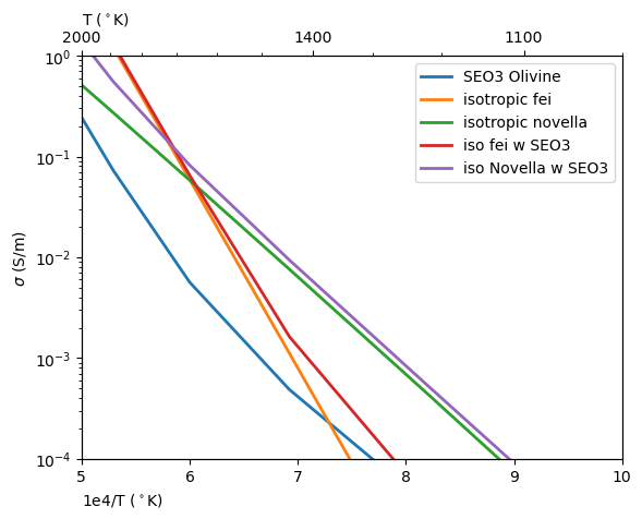
Using these models is now as easy as getting them from the database, sending in the conditions, and plotting the results:
fig, ax = plt.subplots()
linear_major_ticks = np.asarray([2000,1400,1100,900,800,700,600,500,400])
pyhutils.format_ax_arrhenian_space(ax,linear_major_ticks=linear_major_ticks,xlim=[5,10])


fei_ionic_isotropic  = 'isotropic_model:fei_20_ol_ionic[100]+fei_20_ol_ionic[010]+fei_20_ol_ionic[001]'
novella_isotropic    = 'isotropic_model:nv_17_ol[100]+nv_17_ol[010]+nv_17_ol[001]'
fei_ionic_compound   = 'isotropic_model:fei_20_ol_ionic[100]+SEO3_ol+fei_20_ol_ionic[010]+SEO3_ol+fei_20_ol_ionic[001]+SEO3_ol'
novella_wet_compound = 'isotropic_model:nv_17_ol[100]+SEO3_ol+nv_17_ol[010]+SEO3_ol+nv_17_ol[001]+SEO3_ol'
ecmodel = ecdatabase.get_model('SEO3_ol')
c = ecmodel.get_conductivity(**physiochem)
ax.plot(1e4/T,c,label='SEO3 Olivine',linewidth=2)

for label, model_id in zip(['isotropic fei','isotropic novella','iso fei w SEO3', 'iso Novella w SEO3'],
                    [fei_ionic_isotropic,novella_isotropic,fei_ionic_compound,novella_wet_compound ]):
    ecmodel = ecdatabase.get_model(model_id)
    c = ecmodel.get_conductivity(**physiochem)
    ax.plot(1e4/T,c,label=label,linewidth=2)


ax.legend()
ax.set_ylim([1e-4,1])
fig.show()
Water Corrections
Water corrections adjust the conductivity model to account for the presence of water in the system. This is especially important in geophysical contexts where water can dramatically alter the behavior of mineral conductivities. Pyrrhenius provides several water correction models that adjust the conductivity based on the water content in a given system.
Dry Model: copies passed keyword-arguments, setting Cw=0
WaterCorrection: copies passed keyword-arguments, then multiplies the Cw copy by a static factor
WaterPTCorrection: copies passed keyword-arguments, then sets Cw based on a function dependent on T and/or P.
Each of these models can be used to dynamically adjust conductivity based on the amount of water present.
from pyrrhenius.model import WaterCorrection
from pyrrhenius.database import Database

# Initialize database and water-corrected model
ecdatabase = Database()
ecdatabase.create_isotropic_models()
base_model = ecdatabase.get_model('isotropic_model:gar_14_withers_ol[100]+gar_14_withers_ol[010]+gar_14_withers_ol[001]')
water_corrected_model = WaterCorrection(base_model,correction_factor=1/3)

# Define parameters
T = 1200  # Temperature in K
P = 1.5   # Pressure in GPa
Cw = 150   # Water concentration in ppm

# Calculate conductivity with water correction
corrected = water_corrected_model.get_conductivity(T=T, P=P, Cw=Cw)
original  = base_model.get_conductivity(T=T, P=P, Cw=Cw)
print(f"Original Conductivity: {original} S/m")
print(f"Water-Corrected Conductivity: {corrected} S/m")
nan nan
nan nan
nan nan
nan nan
nan nan
nan nan
nan nan
nan nan
nan nan
nan nan
nan nan
nan nan
nan nan
nan nan
nan nan
nan nan
nan nan
nan nan
withers (2012) withers (2012)
ppm ppm
nan nan
withers (2012) withers (2012)
ppm ppm
nan nan
withers (2012) withers (2012)
ppm ppm
nan nan
withers (2012) withers (2012)
ppm ppm
nan nan
withers (2012) withers (2012)
ppm ppm
nan nan
withers (2012) withers (2012)
ppm ppm
nan nan
withers (2012) withers (2012)
ppm ppm
nan nan
withers (2012) withers (2012)
ppm ppm
nan nan
withers (2012) withers (2012)
ppm ppm
nan nan
withers (2012) withers (2012)
ppm ppm
nan nan
withers (2012) withers (2012)
ppm ppm
nan nan
withers (2012) withers (2012)
ppm ppm
nan nan
withers (2012) withers (2012)
ppm ppm
nan nan
withers (2012) withers (2012)
ppm ppm
nan nan
withers (2012) withers (2012)
ppm ppm
nan nan
withers (2012) withers (2012)
ppm ppm
nan nan
withers (2012) withers (2012)
ppm ppm
nan nan
withers (2012) withers (2012)
ppm ppm
nan nan
withers (2012) withers (2012)
ppm ppm
nan nan
withers (2012) withers (2012)
ppm ppm
nan nan
withers (2012) withers (2012)
ppm ppm
nan nan
withers (2012) withers (2012)
ppm ppm
nan nan
withers (2012) withers (2012)
ppm ppm
nan nan
withers (2012) withers (2012)
ppm ppm
nan nan
nan nan
nan nan
nan nan
nan nan
nan nan
nan nan
nan nan
nan nan
nan nan
nan nan
nan nan
nan nan
nan nan
nan nan
nan nan
nan nan
nan nan
nan nan
nan nan
nan nan
nan nan
nan nan
nan nan
nan nan
nan nan
nan nan
nan nan
bell (2003) bell (2003)
ppm ppm
nan nan
bell (2003) bell (2003)
ppm ppm
nan nan
bell (2003) bell (2003)
ppm ppm
nan nan
bell (2003) bell (2003)
ppm ppm
nan nan
bell (2003) bell (2003)
ppm ppm
nan nan
bell (2003) bell (2003)
ppm ppm
nan nan
paterson (1982) paterson (1982)
wtpct wtpct
nan nan
paterson (1982) paterson (1982)
wtpct wtpct
nan nan
paterson (1982) paterson (1982)
wtpct wtpct
nan nan
paterson (1982) paterson (1982)
wtpct wtpct
nan nan
paterson (1982) paterson (1982)
wtpct wtpct
nan nan
paterson (1982) paterson (1982)
wtpct wtpct
nan nan
paterson (1982) paterson (1982)
ppm ppm
nan nan
paterson (1982) paterson (1982)
ppm ppm
nan nan
paterson (1982) paterson (1982)
ppm ppm
nan nan
nan nan
nan nan
nan nan
nan nan
nan nan
nan nan
nan nan
nan nan
nan nan
nan nan
nan nan
nan nan
nan nan
nan nan
nan nan
nan nan
nan nan
nan nan
Libowitzky and rossman (1996) Libowitzky and rossman (1996)
wtpct wtpct
nan nan
Libowitzky and rossman (1996) Libowitzky and rossman (1996)
wtpct wtpct
nan nan
Libowitzky and rossman (1996) Libowitzky and rossman (1996)
wtpct wtpct
nan nan
Libowitzky and rossman (1996) Libowitzky and rossman (1996)
wtpct wtpct
nan nan
Libowitzky and rossman (1996) Libowitzky and rossman (1996)
wtpct wtpct
nan nan
Libowitzky and rossman (1996) Libowitzky and rossman (1996)
wtpct wtpct
nan nan
nan nan
nan nan
nan nan
nan nan
nan nan
nan nan
nan nan
nan nan
nan nan
nan nan
nan nan
nan nan
nan nan
nan nan
nan nan
nan nan
nan nan
nan nan
bell (1995) bell (1995)
ppm ppm
nan nan
bell (1995) bell (1995)
ppm ppm
nan nan
bell (1995) bell (1995)
ppm ppm
nan nan
bell (1995) bell (1995)
ppm ppm
nan nan
bell (1995) bell (1995)
ppm ppm
nan nan
bell (1995) bell (1995)
ppm ppm
nan nan
bell (2003) bell (2003)
ppm ppm
nan nan
bell (2003) bell (2003)
ppm ppm
nan nan
bell (2003) bell (2003)
ppm ppm
nan nan
bell (2003) bell (2003)
ppm ppm
nan nan
bell (2003) bell (2003)
ppm ppm
nan nan
bell (2003) bell (2003)
ppm ppm
nan nan
Johnson and Rossman (2003) Johnson and Rossman (2003)
ppm ppm
nan nan
Johnson and Rossman (2003) Johnson and Rossman (2003)
ppm ppm
nan nan
Johnson and Rossman (2003) Johnson and Rossman (2003)
ppm ppm
nan nan
Johnson and Rossman (2003) Johnson and Rossman (2003)
ppm ppm
nan nan
Johnson and Rossman (2003) Johnson and Rossman (2003)
ppm ppm
nan nan
Johnson and Rossman (2003) Johnson and Rossman (2003)
ppm ppm
nan nan
Original Conductivity: [0.0039755] S/m
Water-Corrected Conductivity: [0.00104387] S/m
Cached Models
Cached Models are designed for performance optimization. When performing multiple conductivity calculations over the same parameter space (such as during large simulations or parameter sweeps), cached models store previous results to avoid redundant calculations. This dramatically improves performance when recalculating conductivity for the same inputs.
Cached models are especially useful in long-running simulations or cases where many conductivity calculations are required over the same parameter range.
from pyrrhenius.model import CachedModel
from pyrrhenius.database import Database
import timeit

# Initialize database and cached model
ecdatabase = Database()
base_model = ecdatabase.get_model('sk17_brine')

cached_model = CachedModel(base_model)

# Define parameters for simulation
T = np.linspace(400,700,num=100) # Temperature in K
P = 1.0   # Pressure in GPa
nacl = 5 # 5% NaCl

def time_base_model():
    return base_model.get_conductivity(T=T, P=P, nacl=nacl)

def time_cached_model():
    return cached_model.get_conductivity(T=T, P=P, nacl=nacl)

base_time = timeit.timeit(time_base_model, number=1000)
print(f"Base Model Time (1000 iterations): {base_time:.6f} seconds")

first_cached_time = timeit.timeit(time_cached_model, number=1)
print(f"Cached Model Time (First Run): {first_cached_time:.6f} seconds")

cached_time = timeit.timeit(time_cached_model, number=1000)
print(f"Cached Model Time (1000 iterations, using cache): {cached_time:.6f} seconds")

base_conductivity = base_model.get_conductivity(T=T, P=P, nacl=nacl)
cached_conductivity = cached_model.get_conductivity(T=T, P=P, nacl=nacl)

print(f"\nBase Model Conductivity: {base_conductivity}")
print(f"Cached Model Conductivity: {cached_conductivity}")

speedup = base_time / cached_time
print(f"\nSpeedup factor (cached vs base): {speedup:.2f}x")
Base Model Time (1000 iterations): 2.375855 seconds
Cached Model Time (First Run): 0.002381 seconds
Cached Model Time (1000 iterations, using cache): 0.000295 seconds

Base Model Conductivity: [12.51336529 13.3152351  14.09626467 ... 39.31318444 39.32998146
 39.34456567]
Cached Model Conductivity: [12.51336529 13.3152351  14.09626467 ... 39.31318444 39.32998146
 39.34456567]

Speedup factor (cached vs base): 8048.07x
In this example, the CachedModel stores the result of the first conductivity calculation. When the same parameters are provided again, it retrieves the result from the cache. For an input array 100 elements long, a speedup greater than 8000x is achieved with the CachedModel.
This is likely an extreme example. For most other models within the Pyrrhenius database, CachedModels are likely to provide a much smaller speedup factor.
Note
Cached models are most effective in simulations with repeated parameter sweeps or when the same conditions are evaluated multiple times.
Warning
CachedModels do not check to see if the input arguments have changed over subsequent calls.
These Special Models provide greater flexibility for dealing with complex real-world scenarios, such as inter-mineral water partitioning corrections.
N-Phase Assemblages
Extremal Bounds
HS + -
Geometric Mixing
Cubes (thin film) and Tubes
Archie’s laws
Modified Archie’s Laws
Effective Medium Theories
Bruggeman symmetric
Maxwell Ghant
Advanced Usage
Inverse Modeling
casting against a conductivity image
binary search
Defining your own Database
Required excel sheet Formatting