Pyrrhenius Quickstart
Basic Usage
The basic workflow of using pyrrhenius is structured like so:
Import necessary modules
import pyrrhenius.database as phsd
Create a pyrrhenius database object
ecdatabase = phsd.Database()
3. Create a pyrrhenius.model.Model object corresponding to the desired model_id. In this case the
model id corresponding to the SEO3 model of olivine (insert citation) is loaded
model = ecdatabase.get_model('SEO3_ol')
Call the
get_conductivity(*args,**kwargs)method on the model with the relevant parameters.
conductivity = model.get_conductivity(T=1000, P=1.0, logfo2=10**-11)
print('*'*20)
print('Calculated conductivity (S/m) at T=1000 K, P=1 GPa,and fO2=10^-11 bars:')
print(conductivity)
********************
Calculated conductivity (S/m) at T=1000 K, P=1 GPa,and fO2=10^-11 bars:
2.7380861532827377e-05
Keywords can be of type float or numpy.ndarray’s. The latter functionality is especially useful for computing conductivities across a vectorized grid.
In this case, using meshgrid on a dummy variable (zz) and a temperature array T creates a temperature array of size (10x10).
import numpy as np

T = np.linspace(500,1500,num=11)
z = np.arange(0,11,1) # dummy variable for demonstration purposes only
tt, xx = np.meshgrid(T,z)
print(tt.shape)
tt
(11, 11)array([[ 500., 600., 700., ..., 1300., 1400., 1500.], [ 500., 600., 700., ..., 1300., 1400., 1500.], [ 500., 600., 700., ..., 1300., 1400., 1500.], ..., [ 500., 600., 700., ..., 1300., 1400., 1500.], [ 500., 600., 700., ..., 1300., 1400., 1500.], [ 500., 600., 700., ..., 1300., 1400., 1500.]])
As long as the input keyword-arguments are directly broadcastable, pyrrhenius can use mixed float and numpy.ndarray objects, vectorizing them as needed.
model.get_conductivity(T=tt, P=1.0, logfo2=10**-11)
array([[1.06820389e-10, 6.71262242e-09, 1.29536636e-07, ...,
        5.52272174e-04, 1.26077070e-03, 2.93431687e-03],
       [1.06820389e-10, 6.71262242e-09, 1.29536636e-07, ...,
        5.52272174e-04, 1.26077070e-03, 2.93431687e-03],
       [1.06820389e-10, 6.71262242e-09, 1.29536636e-07, ...,
        5.52272174e-04, 1.26077070e-03, 2.93431687e-03],
       ...,
       [1.06820389e-10, 6.71262242e-09, 1.29536636e-07, ...,
        5.52272174e-04, 1.26077070e-03, 2.93431687e-03],
       [1.06820389e-10, 6.71262242e-09, 1.29536636e-07, ...,
        5.52272174e-04, 1.26077070e-03, 2.93431687e-03],
       [1.06820389e-10, 6.71262242e-09, 1.29536636e-07, ...,
        5.52272174e-04, 1.26077070e-03, 2.93431687e-03]])
Accessing Database Options
Pyrrhenius currently ships with a .csv database which is loaded by default.
import pyrrhenius.database as phsd

ecdatabase = phsd.Database()
Once the database object has been created, you can use the get_phases(), get_model_list_for_phase(), and the get_model() methods
to specify which model to load.
ecdatabase.get_phases()
['basalt',
 'basaltic melt',
 'brine',
 'clinopyroxene',
 'gabbro',
 'garnet',
 'granite',
 'granulite',
 'olivine',
 'omphacite',
 'orthopyroxene',
 'peridotite',
 'pervoskite',
 'phlogopite',
 'plagioclase',
 'schist',
 'wadsleyite',
 'silicate melt']
ecdatabase.get_model_list_for_phase('granite')
['ks_83_granite',
 'han_23_HD_granite',
 'han_23_QD_low_granite',
 'han_23_QD_high_granite',
 'han_23_QP_low_granite',
 'han_23_QP_high_granite']
ecmodel = ecdatabase.get_model('han_23_HD_granite')
ecmodel
han_23_HD_granite:{9.906(nan) exp( -1.22(0.063)/kT)}
Isotropic Models
The default database comes with a number of anisotropic models, visible as model_id’s with “[xxx]” strings appended to the end. To get an isotropic model, first tell
the database to generate isotropic models via create_isotropic_models(), then examine the available models
before_isotropic_calculation = ecdatabase.get_model_list_for_phase('plagioclase')
ecdatabase.create_isotropic_models()
after_isotropic_calculation = ecdatabase.get_model_list_for_phase('plagioclase')
print('*'*20)
print('Before Isotropic Calculation')
print('*'*20)
print(*before_isotropic_calculation,sep='\n')
print('*'*20)
print('After Isotropic Calculation')
print('*'*20)
print(*after_isotropic_calculation,sep='\n')
nan nan
nan nan
nan nan
nan nan
nan nan
nan nan
nan nan
nan nan
nan nan
nan nan
nan nan
nan nan
nan nan
nan nan
nan nan
nan nan
nan nan
nan nan
withers (2012) withers (2012)
ppm ppm
nan nan
withers (2012) withers (2012)
ppm ppm
nan nan
withers (2012) withers (2012)
ppm ppm
nan nan
withers (2012) withers (2012)
ppm ppm
nan nan
withers (2012) withers (2012)
ppm ppm
nan nan
withers (2012) withers (2012)
ppm ppm
nan nan
withers (2012) withers (2012)
ppm ppm
nan nan
withers (2012) withers (2012)
ppm ppm
nan nan
withers (2012) withers (2012)
ppm ppm
nan nan
withers (2012) withers (2012)
ppm ppm
nan nan
withers (2012) withers (2012)
ppm ppm
nan nan
withers (2012) withers (2012)
ppm ppm
nan nan
withers (2012) withers (2012)
ppm ppm
nan nan
withers (2012) withers (2012)
ppm ppm
nan nan
withers (2012) withers (2012)
ppm ppm
nan nan
withers (2012) withers (2012)
ppm ppm
nan nan
withers (2012) withers (2012)
ppm ppm
nan nan
withers (2012) withers (2012)
ppm ppm
nan nan
withers (2012) withers (2012)
ppm ppm
nan nan
withers (2012) withers (2012)
ppm ppm
nan nan
withers (2012) withers (2012)
ppm ppm
nan nan
withers (2012) withers (2012)
ppm ppm
nan nan
withers (2012) withers (2012)
ppm ppm
nan nan
withers (2012) withers (2012)
ppm ppm
nan nan
nan nan
nan nan
nan nan
nan nan
nan nan
nan nan
nan nan
nan nan
nan nan
nan nan
nan nan
nan nan
nan nan
nan nan
nan nan
nan nan
nan nan
nan nan
nan nan
nan nan
nan nan
nan nan
nan nan
nan nan
nan nan
nan nan
nan nan
bell (2003) bell (2003)
ppm ppm
nan nan
bell (2003) bell (2003)
ppm ppm
nan nan
bell (2003) bell (2003)
ppm ppm
nan nan
bell (2003) bell (2003)
ppm ppm
nan nan
bell (2003) bell (2003)
ppm ppm
nan nan
bell (2003) bell (2003)
ppm ppm
nan nan
paterson (1982) paterson (1982)
wtpct wtpct
nan nan
paterson (1982) paterson (1982)
wtpct wtpct
nan nan
paterson (1982) paterson (1982)
wtpct wtpct
nan nan
paterson (1982) paterson (1982)
wtpct wtpct
nan nan
paterson (1982) paterson (1982)
wtpct wtpct
nan nan
paterson (1982) paterson (1982)
wtpct wtpct
nan nan
paterson (1982) paterson (1982)
ppm ppm
nan nan
paterson (1982) paterson (1982)
ppm ppm
nan nan
paterson (1982) paterson (1982)
ppm ppm
nan nan
nan nan
nan nan
nan nan
nan nan
nan nan
nan nan
nan nan
nan nan
nan nan
nan nan
nan nan
nan nan
nan nan
nan nan
nan nan
nan nan
nan nan
nan nan
Libowitzky and rossman (1996) Libowitzky and rossman (1996)
wtpct wtpct
nan nan
Libowitzky and rossman (1996) Libowitzky and rossman (1996)
wtpct wtpct
nan nan
Libowitzky and rossman (1996) Libowitzky and rossman (1996)
wtpct wtpct
nan nan
Libowitzky and rossman (1996) Libowitzky and rossman (1996)
wtpct wtpct
nan nan
Libowitzky and rossman (1996) Libowitzky and rossman (1996)
wtpct wtpct
nan nan
Libowitzky and rossman (1996) Libowitzky and rossman (1996)
wtpct wtpct
nan nan
nan nan
nan nan
nan nan
nan nan
nan nan
nan nan
nan nan
nan nan
nan nan
nan nan
nan nan
nan nan
nan nan
nan nan
nan nan
nan nan
nan nan
nan nan
bell (1995) bell (1995)
ppm ppm
nan nan
bell (1995) bell (1995)
ppm ppm
nan nan
bell (1995) bell (1995)
ppm ppm
nan nan
bell (1995) bell (1995)
ppm ppm
nan nan
bell (1995) bell (1995)
ppm ppm
nan nan
bell (1995) bell (1995)
ppm ppm
nan nan
bell (2003) bell (2003)
ppm ppm
nan nan
bell (2003) bell (2003)
ppm ppm
nan nan
bell (2003) bell (2003)
ppm ppm
nan nan
bell (2003) bell (2003)
ppm ppm
nan nan
bell (2003) bell (2003)
ppm ppm
nan nan
bell (2003) bell (2003)
ppm ppm
nan nan
Johnson and Rossman (2003) Johnson and Rossman (2003)
ppm ppm
nan nan
Johnson and Rossman (2003) Johnson and Rossman (2003)
ppm ppm
nan nan
Johnson and Rossman (2003) Johnson and Rossman (2003)
ppm ppm
nan nan
Johnson and Rossman (2003) Johnson and Rossman (2003)
ppm ppm
nan nan
Johnson and Rossman (2003) Johnson and Rossman (2003)
ppm ppm
nan nan
Johnson and Rossman (2003) Johnson and Rossman (2003)
ppm ppm
nan nan
********************
Before Isotropic Calculation
********************
yang_11a_plag
yang_12b_plag[100]
yang_12b_plag[010]
yang_12b_plag[001]
Li_18_dry_plag
Li_18_wet_plag
********************
After Isotropic Calculation
********************
yang_11a_plag
yang_12b_plag[100]
yang_12b_plag[010]
yang_12b_plag[001]
Li_18_dry_plag
Li_18_wet_plag
isotropic_model:yang_12b_plag[100]+yang_12b_plag[010]+yang_12b_plag[001]
You should see that calling create_isotropic_models() on the database procedurally creates new model_id’s where multiple crystal directions are present for the same base id. These procedurally generated new models are identified by a prepended isotropic: string. They can now be accessed in the same way as default models
ecmodel = ecdatabase.get_model('isotropic_model:yang_12b_plag[100]+yang_12b_plag[010]+yang_12b_plag[001]')
conductivity = ecmodel.get_conductivity(T=1000, P=1.0)
conductivity
array([0.00061567])
Mixing Models
Pyrrhenius provides several N phase mixing models which are accessed via the mixing module. Since the interfaces for these mixing models
can be different, consult the documentation prior to using them.
import pyrrhenius.mixing as pyhmix

brine_id = 'Li_18_1%plg_brine'
plag_id = 'isotropic_model:yang_12b_plag[100]+yang_12b_plag[010]+yang_12b_plag[001]'

brine_model = ecdatabase.get_model(brine_id)
plag_model  = ecdatabase.get_model(plag_id)
phase_fractions=[0.05,0.95]

# The HashinStrikman mixing model needs to be initialized with a matrix and inclusion ecmodel
hashinshtrikman_matrix = pyhmix.HashinStrickmanBound([brine_model,plag_model])

# The Geometric Average model requires intitialization with a phase and phase fraction list.
geometric_mixed_matrix = pyhmix.GeomAverage([brine_model,plag_model])

# Only the HS model in this example requires a provided phase fraction (0.05), positional argument.
hs_conductivity = hashinshtrikman_matrix.get_conductivity(phase_fractions,T=1000)
gm_conductivity = geometric_mixed_matrix.get_conductivity(phase_fractions,T=1000)

# Also calculate endmember phase conductivities for comparison
plagioclase_conductivity = plag_model.get_conductivity(T=1000)
brine_conductivity        = brine_model.get_conductivity(T=1000)

print(f'HS: {hs_conductivity} GM:{gm_conductivity}')
print(f'Plag: {plagioclase_conductivity} Brine:{brine_conductivity}')
HS: [0.01280826] GM:[0.00084664]
Plag: [0.00061567] Brine:[0.36]
Metadata Access
Most pyrrhenius objects come equipped with a metadata object which describes the source publication, experimental conditions, and calibration settings used to create the model
plag_model.metadata
isotropic_model:yang_12b_plag[100]+yang_12b_plag[010]+yang_12b_plag[001]
:title:None
	author:Xiaozhi Yang+Xiaozhi Yang+Xiaozhi Yang
	year:None
	doi:None
	phase_type:plagioclase
	description:None
	sample_type:None
	equation_form:None
	publication_id:Yang2012+Yang2012+Yang2012
	complete_or_partial_fit:None
	composite_or_single:None
	pressure_average:0.1
	pressure_min:None
	pressure_max:None
	temp_min:473.15
	temp_max:1073.15
	nacl_min:None
	nacl_max:None
	nacl_average:None
	na2o_min:None
	na2o_max:None
	na2o_average:None
	sio2_min:None
	sio2_max:None
	sio2_average:None
	co2_min:None
	co2_max:None
	co2_average:None
	water_min:95.0
	water_max:110.0
	water_average:102.5
	water_calibration:Johnson and Rossman (2003)
	water_units:ppm
	iron_min:None
	iron_max:None
	iron_average:None
	iron_units:nan
	crystal_direction:isotropic
	equation:mixture of:yang_12b_plag[100]*yang_12b_plag[010]*yang_12b_plag[001]
	ec_model:mixture of:yang_12b_plag[100]*yang_12b_plag[010]*yang_12b_plag[001]
metadata objects can be used by the parent model to produce input data representative of the experimental conditions
plag_model.generate_representative_conditions()
{'T': array([ 473.15, 1073.15])}
you can use the output from generate_representative_conditions() to construct your own input arrays, or directly evaluate the condition dictionary within the model itself
condition_dict = plag_model.generate_representative_conditions()
plag_model.get_conductivity(**condition_dict)
array([4.40250906e-11, 1.68569100e-03])
Plotting Utilities
Since most experimental petrologists conduct their parameter fitting in \(\log_{10}(\sigma), \frac{1}{T}\) space, pyrrhenius provides a convenience plotting method to format a matplotlib.Axis for a similar plotting space
import matplotlib.pyplot as plt
import numpy as np
import pyrrhenius.mixing as pyhmix
import pyrrhenius.database as phsd
import pyrrhenius.utils as pyhutils
ecdatabase = phsd.Database()
# endmember models
brine_id = 'Li_18_1%plg_brine'
plag_id = 'Li_18_wet_plag'
brine_model = ecdatabase.get_model(brine_id)
plag_model = ecdatabase.get_model(plag_id)
# The HashinStrikman mixing model needs to be initialized with a matrix and inclusion ecmodel
hashinshtrikman_matrix = pyhmix.HashinStrickmanBound([brine_model,plag_model])
# provide a range of temperature conditions at which to evaluate the models
T = np.linspace(400,1200,num=120)
# Only the HS model in this example requires a provided phase fraction (0.05), positional argument.
hs_5pct = hashinshtrikman_matrix.get_conductivity(0.05,T=T)
hs_1pct = hashinshtrikman_matrix.get_conductivity(0.01,T=T)
# Also calculate endmember phase conductivities for comparison
plagioclase_conductivity = plag_model.get_conductivity(T=T)
brine_conductivity = brine_model.get_conductivity(T=T)
# set up matplotlib plotting
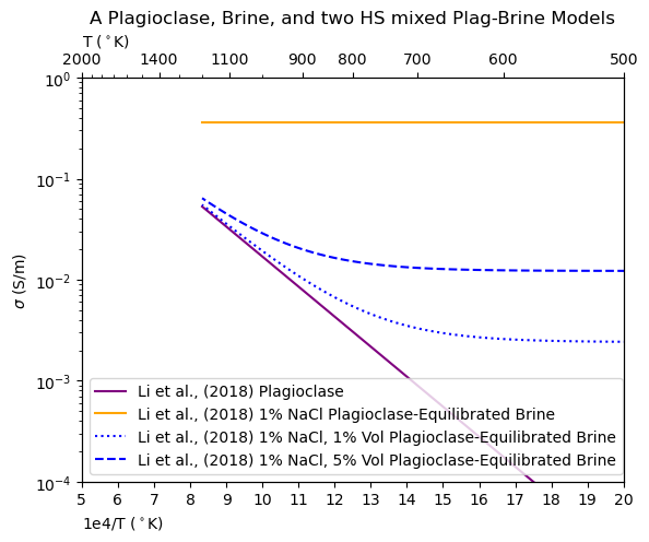
fig, ax = plt.subplots()
linear_major_ticks = np.asarray([2000,1400,1100,900,800,700,600,500,400])
pyhutils.format_ax_arrhenian_space(ax,linear_major_ticks=linear_major_ticks)
ax.plot(1e4/T,plagioclase_conductivity,color='purple',label='Li et al., (2018) Plagioclase')
ax.plot(1e4/T,brine_conductivity,color='orange',label='Li et al., (2018) 1% NaCl Plagioclase-Equilibrated Brine')
ax.plot(1e4/T,hs_1pct,color='blue',label='Li et al., (2018) 1% NaCl, 1% Vol Plagioclase-Equilibrated Brine',linestyle=':')
ax.plot(1e4/T,hs_5pct,color='blue',label='Li et al., (2018) 1% NaCl, 5% Vol Plagioclase-Equilibrated Brine',linestyle='--')
ax.set_title('A Plagioclase, Brine, and two HS mixed Plag-Brine Models')
ax.legend()
fig.show()